The focus now shifts to supply side shocks and a positive shock to labor supply is the first of the supply shocks presented in sections 10 - 14.
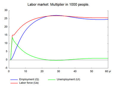
Labor input in ADAM's production function is defined in terms of efficiency corrected labor hours, i.e. as a product of three elements: labor productivity, working hours per year per employed and employment. A change in any of these three components changes the labor input, and the experiments in sections 10 - 12 present a shock to each of the three elements. In all cases, production increases in the medium and long run. In this section, we consider the effect of a permanent increase in the number of people in the work force caused by a reduction of 1 percent of total employment in the number of people outside the labor force not receiving transfers. The work force increases approximately by 27000 people. (See experiment)
Table 10. The effect of a permanent increase in labor supply
| 1. yr | 2. yr | 3. yr | 4. yr | 5. yr | 10. yr | 15. yr | 20. yr | 25. yr | 30. yr | ||
| Million 2010-Dkr. | |||||||||||
| Priv. consumption | fCp | 950 | 1776 | 2420 | 2617 | 2549 | 107 | -2765 | -4494 | -5067 | -4913 |
| Pub. consumption | fCo | 0 | 0 | 1 | 3 | 5 | 16 | 26 | 31 | 35 | 38 |
| Investment | fI | 672 | 1764 | 2682 | 3189 | 3475 | 3269 | 2465 | 2350 | 2767 | 3326 |
| Export | fE | 612 | 1612 | 2804 | 4162 | 5644 | 13582 | 20557 | 25622 | 28749 | 30404 |
| Import | fM | 599 | 1333 | 1932 | 2255 | 2462 | 2895 | 3393 | 4289 | 5275 | 6085 |
| GDP | fY | 1633 | 3804 | 5879 | 7569 | 8999 | 13581 | 16175 | 18346 | 20223 | 21708 |
| 1000 Persons | |||||||||||
| Employment | Q | 1,34 | 3,64 | 6,17 | 8,63 | 10,90 | 19,14 | 23,47 | 25,89 | 26,98 | 27,00 |
| Unemployment | Ul | 13,73 | 11,53 | 10,23 | 9,00 | 7,86 | 3,75 | 1,59 | 0,39 | -0,16 | -0,16 |
| Percent of GDP | |||||||||||
| Pub. budget balance | Tfn_o/Y | -0,15 | -0,11 | -0,04 | 0,05 | 0,13 | 0,36 | 0,47 | 0,56 | 0,64 | 0,71 |
| Priv. saving surplus | Tfn_hc/Y | 0,12 | 0,05 | -0,04 | -0,12 | -0,17 | -0,18 | -0,06 | 0,01 | 0,04 | 0,03 |
| Balance of payments | Enl/Y | -0,03 | -0,06 | -0,08 | -0,07 | -0,04 | 0,17 | 0,40 | 0,57 | 0,68 | 0,75 |
| Foreign receivables | Wnnb_e/Y | 0,03 | 0,06 | 0,07 | 0,08 | 0,13 | 0,86 | 2,46 | 4,55 | 6,81 | 9,03 |
| Bond debt | Wbd_os_z/Y | 0,15 | 0,26 | 0,30 | 0,26 | 0,15 | -1,03 | -2,66 | -4,44 | -6,31 | -8,19 |
| Percent | |||||||||||
| Capital intensity | fKn/fX | -0,08 | -0,17 | -0,25 | -0,31 | -0,35 | -0,47 | -0,57 | -0,67 | -0,72 | -0,73 |
| Labour intensity | hq/fX | -0,03 | -0,07 | -0,09 | -0,09 | -0,09 | -0,05 | -0,02 | 0,00 | 0,02 | 0,02 |
| User cost | uim | -0,11 | -0,25 | -0,38 | -0,49 | -0,59 | -0,96 | -1,14 | -1,19 | -1,17 | -1,11 |
| Wage | lna | -0,25 | -0,67 | -1,02 | -1,32 | -1,58 | -2,42 | -2,74 | -2,77 | -2,65 | -2,47 |
| Consumption price | pcp | -0,10 | -0,24 | -0,37 | -0,49 | -0,60 | -1,02 | -1,26 | -1,38 | -1,40 | -1,35 |
| Terms of trade | bpe | -0,07 | -0,16 | -0,25 | -0,32 | -0,39 | -0,64 | -0,76 | -0,79 | -0,76 | -0,72 |
| Percentage-point | |||||||||||
| Consumption ratio | bcp | -0,13 | -0,09 | -0,03 | 0,03 | 0,07 | 0,04 | -0,10 | -0,20 | -0,25 | -0,26 |
| Wage share | byw | -0,08 | -0,21 | -0,30 | -0,36 | -0,40 | -0,49 | -0,47 | -0,40 | -0,33 | -0,27 |
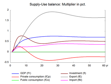
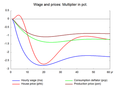
The increased labor supply is not automatically employed at once as there is no demand side response, so unemployment increases. The higher unemployment reduces the growth of wages and prices. The decline in prices relative to the baseline improves competitiveness, as a result production and exports increase and gradually pull the extra labor force into employment. Employment increases until the additional labor force is employed and the rate of unemployment is back at its structural level.
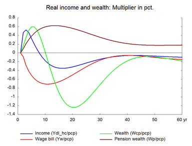
The positive effect on employment, the negative effect on wages and the positive effect on exports is permanent. Private consumption rises in the short run as the unemployed people receive unemployment benefits and other social benefits. The long term impact on private consumption is negative due to the negative real wage effect.▼ Real wage effect arises because wages increase/decrease more than the general price levels due to the deadweight from the non-responding exogenous import prices. This creates a positive/negative real wage effect, terms of trade and real disposable income and private consumption increase/decrease permanently. When domestic demand falls the export needs to increase even more for the extra supply of workers to be soaked up in the economy. For this to happend, terms of trade need to be even better. Thus, wage will have to decrease more.
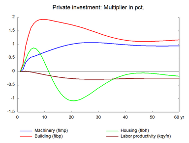
Overall, there is a positive effect on production in the long run because of the permanent increase in employment. There is also a permanent change in the relative prices of production factors, as labor becomes relatively cheaper compared to the partly imported capital. This implies a substitution effect.▼ A substitution effect arises when a change in the relative prices of factors induces producers to use more of a relatively cheaper factor and less of a relatively more expensive factor. Consequently, the substitution of labor for capital making production more labor intensive and reducing labor productivity. The substitution effect offsets part of the increase in production.
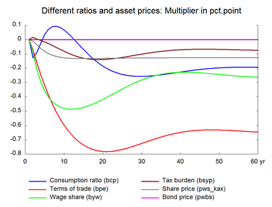
In contrast to section 1, the wage share falls permanently, i.e. the distribution of income changes permanently in favour of capital. Wage relative to user cost falls in the long run because investment prices fall less than wages due to the deadweight from import prices.
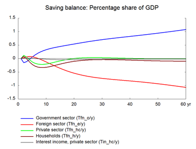
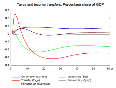
There is a significant positive effect on public budget in the long term, because the nominal fall in revenues is larger than the nominal fall in expenditures. Transfer payments and public wage-expenses decline as hourly wages fall. Other public expenditures also fall as prices fall. On the revenue side, taxes on personal income fall when hourly wages fall. But the number of tax payers increases and this offsets some of the fall in tax revenue.
The negative long-term impact on consumption can be seen in relation to two things: Firstly the absence of a fiscal reaction function and secondly the size of the foreign trade elasticities. See section 19 for a scenario with a fiscal reaction function and section 20 for a scenario with higher export price elasticity.
In general, a permanent increase in the labor force has a permanent positive effect on employment and output. The higher tax revenues provide a potential for higher public spending or lower taxes, which could boost domestic demand and moderate the need for higher exports.
Figure 10. The effect of a permanent increase in labor supply with 27000 people
