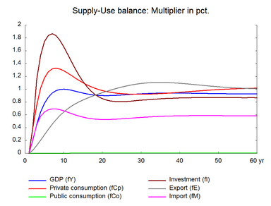
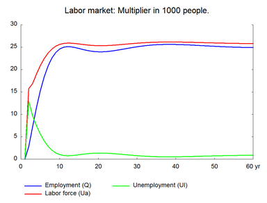
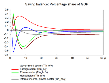
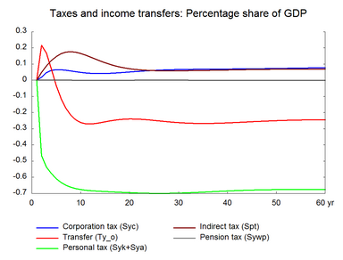
Increasing the labor supply has a permanent positive effect on the public budget balance. The additional public savings can be used to increase spending or to reduce tax rates in order to create expansionary effects in the economy. Table 19 presents the effect of a permanent increase in labor supply accompanied by a permanent decrease in income tax rates. As in section 10, the number of people outside the labor force not receiving transfers is reduced by 1 percent of total employment - approximately 27.000 people and, in contrast to section 10, central government income tax rates are reduced permanently by 6.16 percent (e.g. from 15 to 14.08 per cent) to balance the public budget in the long run. (See experiment)
Table 19. The effect of a permanent increase in labor supply, balanced budget
| 1. yr | 2. yr | 3. yr | 4. yr | 5. yr | 10. yr | 15. yr | 20. yr | 25. yr | 30. yr | ||
| Million 2010-Dkr. | |||||||||||
| Priv. consumption | fCp | 3542 | 6773 | 9329 | 10967 | 12038 | 12775 | 11736 | 11415 | 11817 | 12668 |
| Pub. consumption | fCo | 0 | 0 | 1 | 3 | 4 | 12 | 17 | 20 | 21 | 22 |
| Investment | fI | 1908 | 4715 | 6745 | 7776 | 8388 | 7710 | 5608 | 4841 | 5077 | 5634 |
| Export | fE | 506 | 1300 | 2190 | 3153 | 4134 | 8283 | 11044 | 13385 | 15648 | 17627 |
| Import | fM | 2096 | 4268 | 5791 | 6577 | 7082 | 7305 | 6795 | 7020 | 7784 | 8719 |
| GDP | fY | 3900 | 8550 | 12437 | 15246 | 17360 | 21195 | 21241 | 22199 | 24268 | 26662 |
| 1000 Persons | |||||||||||
| Employment | Q | 2,81 | 7,22 | 11,54 | 15,29 | 18,38 | 24,98 | 24,48 | 23,96 | 24,49 | 25,21 |
| Unemployment | Ul | 12,94 | 9,65 | 7,46 | 5,60 | 4,07 | 0,84 | 1,12 | 1,37 | 1,10 | 0,73 |
| Percent of GDP | |||||||||||
| Pub. budget balance | Tfn_o/Y | -0,53 | -0,42 | -0,28 | -0,15 | -0,05 | 0,07 | -0,01 | -0,05 | -0,05 | -0,03 |
| Priv. saving surplus | Tfn_hc/Y | 0,42 | 0,19 | -0,04 | -0,20 | -0,30 | -0,34 | -0,14 | -0,04 | -0,01 | -0,01 |
| Balance of payments | Enl/Y | -0,11 | -0,24 | -0,31 | -0,35 | -0,36 | -0,26 | -0,15 | -0,09 | -0,06 | -0,04 |
| Foreign receivables | Wnnb_e/Y | -0,12 | -0,41 | -0,76 | -1,13 | -1,48 | -2,76 | -3,16 | -3,10 | -2,89 | -2,64 |
| Bond debt | Wbd_os_z/Y | 0,45 | 0,80 | 1,01 | 1,11 | 1,12 | 0,73 | 0,55 | 0,67 | 0,81 | 0,86 |
| Percent | |||||||||||
| Capital intensity | fKn/fX | -0,16 | -0,34 | -0,44 | -0,48 | -0,48 | -0,24 | -0,04 | -0,02 | -0,07 | -0,11 |
| Labour intensity | hq/fX | -0,08 | -0,15 | -0,19 | -0,19 | -0,18 | -0,09 | -0,06 | -0,07 | -0,07 | -0,07 |
| User cost | uim | -0,11 | -0,23 | -0,33 | -0,41 | -0,48 | -0,60 | -0,63 | -0,66 | -0,70 | -0,71 |
| Wage | lna | -0,24 | -0,60 | -0,87 | -1,06 | -1,20 | -1,39 | -1,41 | -1,49 | -1,57 | -1,58 |
| Consumption price | pcp | -0,10 | -0,21 | -0,31 | -0,39 | -0,45 | -0,57 | -0,62 | -0,68 | -0,74 | -0,78 |
| Terms of trade | bpe | -0,07 | -0,15 | -0,21 | -0,26 | -0,29 | -0,37 | -0,39 | -0,42 | -0,44 | -0,45 |
| Percentage-point | |||||||||||
| Consumption ratio | bcp | -0,43 | -0,26 | -0,07 | 0,06 | 0,15 | 0,24 | 0,12 | 0,04 | 0,01 | 0,00 |
| Wage share | byw | -0,11 | -0,24 | -0,31 | -0,34 | -0,34 | -0,28 | -0,26 | -0,28 | -0,28 | -0,27 |
The lower income tax rates reduce government revenues and public savings fall. In the short run, the negative effect on the public budget dominates, but in the long term, public budget and debt constitute the same ratios of GDP as in the baseline.
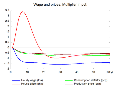
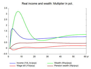
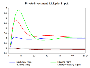
The higher labor supply is not immediately employed, so unemployment increases in the short run. The higher unemployment exerts a downward pressure on wages and prices which improves competitiveness. This makes exports stimulate production and employment. The expansionary effect is reinforced by higher private consumption, which peaks after five years. The higher consumption reflects that the lower income tax rates have increased disposable income. The stronger domestic demand makes unemployment fall more sharply than in section 10. Employment keeps increasing until the additional labor force is employed and the rate of unemployment has returned to its baseline. The higher production increases the capital stock and investments permanently. Imports also increase permanently to meet the higher domestic demand.
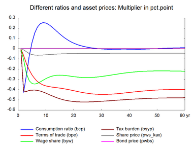
When the government budget is unchanged as a share of GDP, the balance of payment is also unchanged in the long run as indicated in table 19. Moreover, in this balanced-budget experiment net exports remain fairly unchanged implying that the volume change in net exports is balanced by the price change. This balancing of nominal exports and imports is illustrated in figure 19, where the percentage increase in real exports minus the percentage increase in real imports, cf. first diagram on the left hand side, is equal to the percentage deterioration in the terms of trade, cf. last diagram on the right hand side.
In the long run, the need for lower wages to boost competitiveness will moderate the increase in real income and private consumption. The initial consumption boom raises the demand for dwellings, housing investment and house price increase, and the higher housing wealth has a certain feed-back effect on private consumption. Moreover, the short-run expansion of the housing capital is stronger than the long run effect. The excess supply of houses created in the medium run reduces house prices and the housing investment is adjusted downwards before the housing market reaches its equilibrium.
Taking this section 19 together with section 10, illustrates the importance of the budget constraint. Spending the supply-driven improvement of public finances on fiscal easing makes employment increase faster in section 19 than in section 10, and the long-run need for higher exports and improved competitiveness is lower in section 19. In section 10, the additional supply was used to boost public finances and net exports. In section 19, it is primarily used to increase domestic consumption. Making the public sector spend its additional revenues resembles an introduction of Say’s law.
In a closed economy, spending the full-structural-employment GDP on consumption and investment would be enough to secure full structural employment. However, in an open economy a share of domestic demand will be met by higher imports, and exports will have to increase accordingly. Consequently, we still get an export increase in section 19, but as we have seen, the export increase is smaller than in section 10. In real terms, the long-run increase of exports in ADAM will always match full-structural-employment GDP plus imports minus domestic demand. And in this section 19, the increase of exports will also match the increase of imports in nominal terms, because the constant public budget plus the private consumption function makes the impact on domestic demand match the impact on GDP in nominal terms.
Figure 19. The effect of a permanent increase in labor supply, balanced budget
