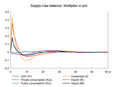
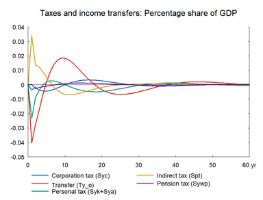
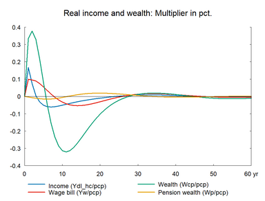
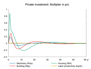
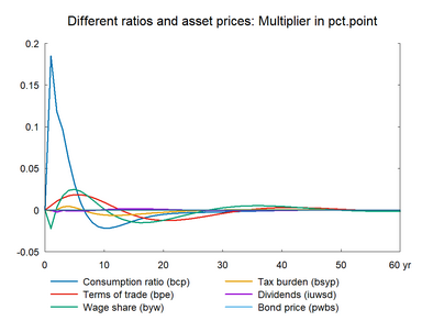
All the previous sections have highlighted the role that consumption and wage equations play in ADAM in achieving stability after the economy have been displaced from equilibrium. In the present and subsequent section, we introduce a shock to these equations one by one. This section presents the effect of a temporary increase in the propensity to consume. The shock to private consumption is made by a one off change in the constant of the consumption function, which directly influences consumption. Private consumption is increased in year one by 0.1 percent of GDP. (See experiment)
Table 16. The effect of a temporary exogenous increase in private consumption
| 1. yr | 2. yr | 3. yr | 4. yr | 5. yr | 10. yr | 15. yr | 20. yr | 25. yr | 30. yr | ||
| Million 2010-Dkr. | |||||||||||
| Priv. consumption | fCp | 3896 | 2377 | 1739 | 1015 | 438 | -693 | -592 | -351 | -150 | 2 |
| Pub. consumption | fCo | -127 | -111 | -87 | -57 | -28 | 43 | 34 | 11 | -3 | -9 |
| Investment | fI | 2705 | 1492 | 660 | 301 | -41 | -759 | -428 | 0 | 205 | 228 |
| Export | fE | -102 | -256 | -365 | -454 | -520 | -525 | -60 | 423 | 603 | 466 |
| Import | fM | 2709 | 1363 | 611 | 222 | -99 | -615 | -368 | -53 | 134 | 183 |
| GDP | fY | 3846 | 2250 | 1404 | 614 | -55 | -1398 | -762 | 56 | 445 | 434 |
| 1000 Persons | |||||||||||
| Employment | Q | 2.68 | 1.97 | 1.42 | 0.76 | 0.13 | -1.41 | -0.79 | 0.11 | 0.51 | 0.47 |
| Unemployment | Ul | -1.51 | -0.91 | -0.67 | -0.35 | -0.04 | 0.70 | 0.39 | -0.05 | -0.26 | -0.24 |
| Percent of GDP | |||||||||||
| Pub. budget balance | Tfn_o/Y | 0.10 | 0.06 | 0.05 | 0.03 | 0.01 | -0.03 | -0.02 | 0.00 | 0.00 | 0.01 |
| Priv. saving surplus | Tfn_hc/Y | -0.22 | -0.13 | -0.08 | -0.05 | -0.02 | 0.04 | 0.02 | 0.00 | 0.00 | 0.00 |
| Balance of payments | Enl/Y | -0.12 | -0.06 | -0.04 | -0.02 | -0.01 | 0.00 | 0.00 | 0.00 | 0.00 | 0.00 |
| Foreign receivables | Wnnb_e/Y | -0.19 | -0.21 | -0.22 | -0.22 | -0.22 | -0.15 | -0.11 | -0.09 | -0.06 | -0.04 |
| Bond debt | Wbd_os_z/Y | -0.11 | -0.15 | -0.19 | -0.21 | -0.21 | -0.07 | 0.06 | 0.09 | 0.06 | 0.02 |
| Percent | |||||||||||
| Capital intensity | fKn/fX | -0.10 | -0.03 | 0.01 | 0.04 | 0.06 | 0.06 | 0.00 | -0.02 | -0.03 | -0.01 |
| Labour intensity | hq/fX | -0.04 | -0.01 | 0.00 | 0.01 | 0.01 | 0.00 | 0.00 | 0.00 | 0.00 | 0.00 |
| User cost | uim | 0.01 | 0.01 | 0.02 | 0.02 | 0.03 | 0.01 | -0.01 | -0.02 | -0.02 | -0.01 |
| Wage | lna | 0.03 | 0.05 | 0.07 | 0.08 | 0.08 | 0.03 | -0.03 | -0.05 | -0.03 | -0.01 |
| Consumption price | pcp | 0.01 | 0.01 | 0.02 | 0.03 | 0.03 | 0.02 | 0.00 | -0.02 | -0.02 | -0.01 |
| Terms of trade | bpe | 0.01 | 0.01 | 0.01 | 0.02 | 0.02 | 0.01 | -0.01 | -0.01 | -0.01 | 0.00 |
| Percentage-point | |||||||||||
| Consumption ratio | bcp | 0.18 | 0.12 | 0.10 | 0.06 | 0.03 | -0.02 | -0.01 | -0.01 | 0.00 | 0.00 |
| Wage share | byw | -0.02 | 0.00 | 0.02 | 0.02 | 0.02 | 0.00 | -0.01 | -0.01 | 0.00 | 0.00 |
The shock to private consumption initially works in the same way as a shock to public consumption. Higher private consumption boosts domestic demand; hence private production and employment increase. This creates additional demand for consumption and investment. Imports also increase in the short run as part of the higher domestic demand is met through imports. The higher employment stimulates wage growth and prices and competitiveness fall, leading to a fall in exports.
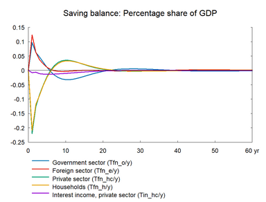
The effect on employment, production, private and public saving balances, etc is temporary reflecting that it is a temporary demand shock and the consumption function is an error correction equation that adjusts back to the long term value. Consumption keeps adjusting until the ratio between wealth and income is back to the baseline value. The adjustment of consumption, however, takes a long time. Consumption remains above the baseline for a few years followed by a long period below the baseline. The latter period restores wealth and the ratio between income and wealth will return to the equilibrium value, and consumption will return to the baseline. The initial stimulus to economic activity is sufficient to stimulate wages and hence prices, and it takes time for the higher wage rate to return to the baseline.
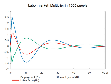
The crowding out process is illustrated by the fluctuation in unemployment. Unemployment falls initially and this pushes up the wage rate slightly. In year 2, the consumption shock disappears and the higher wage pulls unemployment up. Unemployment has to be above the baseline for a while in order to pull the wage rate back down to the baseline. Basically, wages fall relative to the baseline as long as unemployment is above the baseline. So that both unemployment and wage will fluctuate around the baseline on their way back to the baseline. This reflects that the link between unemployment and wage change makes unemployment fluctuate, while the area between unemployment and the baseline converges to zero. It is noted that the basic adjustment process is similar to the adjustment after an overheating of the economy.
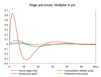
The experiment also makes the housing market fluctuate. In the first year, house prices increase sharply because of the higher consumption and this raises housing wealth. Higher housing wealth in turn expands private consumption. The immediate positive impact on house prices triggers a higher Tobin’s q and housing investment increases. Later on, the higher housing capital reduces house price and Tobin's q after the initial increase in consumption has disappeared. The lower house price drives housing investment and hence housing capital down. In this way, housing capital returns to the baseline and the area between Tobin's q and the baseline converges to zero just like the area between investments and its baseline. In general, the temporary shock to consumption starts an adjustment process with fluctuations.
Figure 16. The effect of a temporary exogenous increase in private consumption
